8 Eigenvectors and eigenvalues: practical solutions
TODO change this lecture to:
- QR with gram-schmidt
- power iteration and inverse power iteration
- orthogonal vs orthonormal
In the previous lecture, we defined the eigenvalue problem for a matrix \(A\): Finding numbers \(\lambda\) (eigenvalues) and vectors \(\vec{x}\) (eigenvectors) which satisfy the equation: \[\begin{equation} A \vec{x} = \lambda \vec{x}. \end{equation}\] We saw one starting point for finding eigenvalues is to find the roots of the characteristic equation: a polynomial of degree \(n\) for an \(n \times n\) matrix \(A\). But we already have seen that this approach will be infeasible for large matrices. Instead, we will find a sequence of similar matrices to \(A\) such that we can read off the eigenvalues from the final matrix.
In equations, we can say our “grand strategy” is to find a sequence of matrices \(P_1, P_2, \ldots\) to form a sequence of matrices: \[\begin{equation} \label{eq:similarity_transform} A, P_1^{-1} A P, P_2^{-1} P_1^{-1} A P_1 P_2, P_3^{-1} P_2^{-1} P_1^{-1} A P_1 P_2 P_3, \ldots \end{equation}\] Our aim is to get all the way to a simple matrix where we read off the eigenvalues and eigenvectors.
For example, if at level \(m\), say, we have transformed \(A\) into a diagonal matrix the eigenvalues are the diagonal of the matrix \[\begin{equation*} P_m^{-1} P_{m-1}^{-1} \cdots P_2^{-1} P_1^{-1} A P_1 P_2 \cdots P_{m-1} P_m, \end{equation*}\] and the eigenvectors are the columns of the matrix \[\begin{equation*} S_m = P_1 P_2 \cdots P_{m-1} P_m. \end{equation*}\] Sometimes, we only want to compute eigenvalues, and not eigenvectors, then it is sufficient to transform the matrix to be triangular (either upper or lower triangular). Then, we can read off that the eigenvalues are the diagonal entries (see ?exm-eigenvalue-triangular).
Remark 8.1. In the example below, and many others, we see that we typically want the matrices \(P_j\) to be orthogonal. A (real-valued) matrix \(Q\) is orthogonal if \(Q^T Q = I_n\).
Orthogonal matrices have the nice property that \(Q^{-1} = Q^T\) so we can very easily compute their inverse! They also always have determinant 1 and their columns are orthonormal too. Finally, we can apply them (or their inverses) without worrying about adding extra problems from finite precision.
Examples of orthogonal matrices include matrices which describe rotations and reflections.
8.1 QR algorithm
The QR algorithm is an iterative method for computing eigenvalues and eigenvectors. At each step a matrix is factored into a product in a similar fashion to LU factorisation (?sec-lu-factorisation). In this case, we factor a matrix, \(A\) into a product of an orthgonal matrix, \(Q\), and an upper triangular matrix, \(R\): \[ A = Q R. \] This is QR factorisation.
Given a matrix \(A\), the algorithm repeatedly applies QR factorisation. First, we set \(A^{(0)} = A\), then we successively perform for \(k=0, 1, 2, \ldots\):
Compute the QR factorisation of \(A^{(k)}\) into an orthogonal part and upper triangular part \[ A^{(k)} = Q^{(k)} R^{(k)}; \]
Update the matrix \(A^{(k+1)}\) recombining \(Q\) and \(R\) in the reverse order: \[ A^{(k+1)} = R^{(k)} Q^{(k)}. \]
As we take more and more steps, we hope that \(A^{(k)}\) converges to an upper triangular matrix whose diagonal entries are the eigenvalues of the original matrix.
Rearranging the first step within each iteration, we see that \[ R^{(k)} = (Q^{(k)})^{-1} A^{(k)} = (Q^{(k)})^T A^{(k)}. \] Substituting this value of \(R^{(k)}\) into the second step gives \[ A^{(k+1)} = (Q^{(k)})^{-1} A^{(k)} Q^{(k)}, \] and we see that at each step we are finding a sequence of similar matrices, all with the same eigenvalues ({?thm-XX}). We can additionally find the eigenvectors of \(A\) by forming the product \[ Q = Q^{(1)} Q^{(2)} \cdots Q^{(m)}. \]
The hard part of the method is compute the QR factorisation. One classical way to get a QR factorisation is to use the Gram-Schmidt process. In general, Gram-Schmidt is used for take a sequence of vectors and forming a new sequence which is orthogonal. We can apply this to the columns of \(A\) to form an orthogonal matrix. It turns out that if we track this process as a matrix-matrix product we find that the other factor is upper triangular.
8.1.1 The Gram-Schmidt process
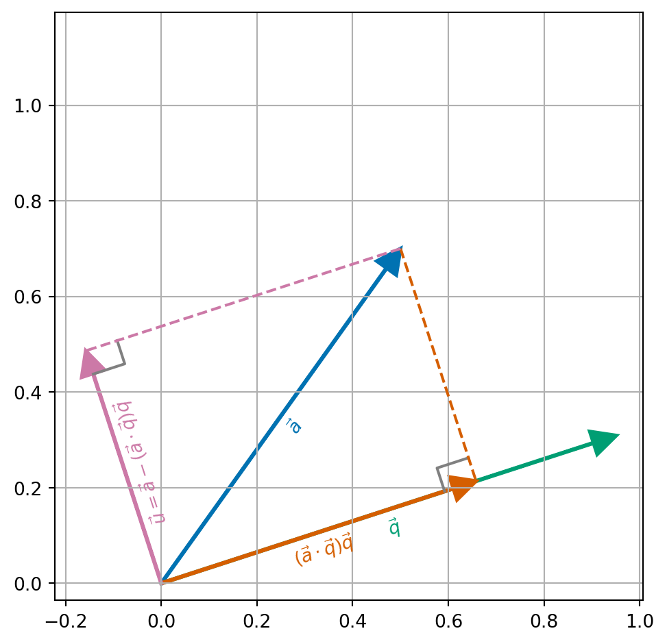
The key idea is shown in Figure 8.1. Given a vector \(\vec{a}\) (blue) and a vector \(\vec{q}\) (green) with length 1. We can compute the projection of \(\vec{a}\) onto the direction \(\vec{q}\) (orange) by \[\begin{align*} (\vec{a} \cdot \vec{q}) \vec{q}. \end{align*}\] If we subtract this term from \(\vec{a}\). We end up with a vector \(\vec{u}\) with \(\vec{u} \cdot \vec{q} = 0\). The difference \(\vec{u}\) is given by \[\begin{align*} \vec{u} = \vec{a} - (\vec{a} \cdot \vec{q}) \vec{q}, \end{align*}\] and we can compute that \[\begin{align*} \vec{u} \cdot \vec{q} & = (\vec{a} - (\vec{a} \cdot \vec{q}) \vec{q}) \cdot \vec{q} \\ & = (\vec{a} \cdot \vec{q}) - (\vec{a} \cdot \vec{q}) (\vec{q} \cdot \vec{q}) && \text{(properties of scalar product)}\\ & = (\vec{a} \cdot \vec{q}) - (\vec{a} \cdot \vec{q}) && \text{(since $\| \vec{q} \| = 1$)} \\ & = 0. \end{align*}\]
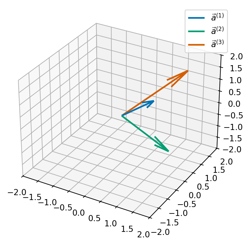
Example 8.1 Consider the sequence of vectors \[\begin{equation*} \vec{a}^{(1)} = \begin{pmatrix} 1 \\ 0 \\ 1 \end{pmatrix}, \vec{a}^{(2)} = \begin{pmatrix} 2 \\ -1 \\ 0 \end{pmatrix}, \vec{a}^{(3)} = \begin{pmatrix} 1 \\ 2 \\ 1 \end{pmatrix}. \end{equation*}\] We will manipulate these vectors to form three vectors which are orthonormal.
First, we set \(\vec{q}^{(1)} = \vec{a}^{(1)} / \| \vec{a}^{(1)} \|\): \[\begin{align*} \| \vec{a}^{(1)} \| = \sqrt{1^2 + 0^2 + 1^2} = \sqrt{2}, \end{align*}\] so \[\begin{equation*} \vec{q}^{(1)} = \begin{pmatrix} \frac{1}{\sqrt{2}} \\ 0 \\ \frac{1}{\sqrt{2}} \end{pmatrix}. \end{equation*}\]
Second, we want to find \(\vec{q}^{(2)}\) which must satisfy that \(\vec{q}^{(2)} \cdot \vec{q}^{(1)} = 0\). We can do this by subtracting form \(\vec{a}^{(2)}\) the portion of \(\vec{a}^{(2)}\) which points in the direction \(\vec{q}^{(1)}\). We call this \(\vec{u}^{(2)}\): \[\begin{align*} \vec{u}^{(2)} & = \vec{a}^{(2)} - \left(\vec{a}^{(2)} \cdot \vec{q}^{(1)} \right) \vec{q}^{(1)} \\ & = \begin{pmatrix} 2 \\ -1 \\ 0 \end{pmatrix} - \left(\begin{pmatrix} 2 \\ -1 \\ 0 \end{pmatrix} \cdot \begin{pmatrix} \frac{1}{\sqrt{2}} \\ 0 \\ \frac{1}{\sqrt{2}} \end{pmatrix} \right) \begin{pmatrix} \frac{1}{\sqrt{2}} \\ 0 \\ \frac{1}{\sqrt{2}} \end{pmatrix} \\ & = \begin{pmatrix} 2 \\ -1 \\ 0 \end{pmatrix} - \frac{2}{\sqrt{2}} \begin{pmatrix} \frac{1}{\sqrt{2}} \\ 0 \\ \frac{1}{\sqrt{2}} \end{pmatrix} \\ & = \begin{pmatrix} 2 - \frac{2}{\sqrt{2}} \frac{1}{\sqrt{2}} \\ -1 - \frac{2}{\sqrt{2}} 0 \\ 0 - \frac{2}{\sqrt{2}} \frac{1}{\sqrt{2}} \end{pmatrix} = \begin{pmatrix} 1 \\ -1 \\ -1 \end{pmatrix}. \end{align*}\] We then normalise \(\vec{u}^{(2)}\) to get a unit-length vector \(q^{(2)}\): \[\begin{align*} \vec{q}^{(2)} & = \vec{u}^{(2)} / \| \vec{u}^{(2)} \| = \begin{pmatrix} \frac{1}{\sqrt{3}} \\ \frac{-1}{\sqrt{3}} \\ \frac{-1}{\sqrt{3}} \end{pmatrix}. \end{align*}\]
Third, we will find \(q^{(3)}\) which we need to check satisfies \(\vec{q}^{(3)} \cdot \vec{q}^{(2)} = 0\) and \(\vec{q}^{(3)} \cdot \vec{q}^{(1)} = 0\). We can do this by subtracting from \(\vec{a}^{(3)}\) the portion of \(\vec{a}^{(3)}\) which points in the direction \(\vec{q}^{(1)}\) and the portion of \(\vec{a}^{(3)}\) which points in the direction \(\vec{q}^{(2)}\). We call this term \(\vec{u}^{(3)}\) \[\begin{align*} \vec{u}^{(3)} & = \vec{a}^{(3)} - \left(\vec{a}^{(3)} \cdot \vec{q}^{(1)} \right) \vec{q}^{(1)} - \left( \vec{a}^{(3)} \cdot \vec{q}^{(2)} \right) \vec{q}^{(2)} \\ & = \begin{pmatrix} 1 \\ 2 \\ 1 \end{pmatrix} - \left( \begin{pmatrix} 1 \\ 2 \\ 1 \end{pmatrix} \cdot \begin{pmatrix} \frac{1}{\sqrt{2}} \\ 0 \\ \frac{1}{\sqrt{2}} \end{pmatrix} \right) \begin{pmatrix} \frac{1}{\sqrt{2}} \\ 0 \\ \frac{1}{\sqrt{2}} \end{pmatrix} - \left( \begin{pmatrix} 1 \\ 2 \\ 1 \end{pmatrix} \cdot \begin{pmatrix} \frac{1}{\sqrt{3}} \\ \frac{-1}{\sqrt{3}} \\ \frac{-1}{\sqrt{3}} \end{pmatrix} \right) \begin{pmatrix} \frac{1}{\sqrt{3}} \\ \frac{-1}{\sqrt{3}} \\ \frac{-1}{\sqrt{3}} \end{pmatrix} \\ & = \begin{pmatrix} 1 \\ 2 \\ 1 \end{pmatrix} - \left( \frac{2}{\sqrt{2}} \right) \begin{pmatrix} \frac{1}{\sqrt{2}} \\ 0 \\ \frac{1}{\sqrt{2}} \end{pmatrix} - \left( \frac{-2}{\sqrt{3}} \right) \begin{pmatrix} \frac{1}{\sqrt{3}} \\ \frac{-1}{\sqrt{3}} \\ \frac{-1}{\sqrt{3}} \end{pmatrix} \\ & = \begin{pmatrix} 1 \\ 2 \\ 1 \end{pmatrix} - \begin{pmatrix} 1 \\ 0 \\ 1 \end{pmatrix} - \begin{pmatrix} -2/3 \\ 2/3 \\ 2/3 \end{pmatrix} = \begin{pmatrix} 2/3 \\ 4/3 \\ -2/3. \end{pmatrix}. \end{align*}\] Again, we normalise \(\vec{u}^{(3)}\) to get \(\vec{q}^{(3)}\): \[\begin{align*} \| \vec{u}^{(3)} \| & = \sqrt{(2/3)^2 + (4/3)^2 + (-2/3)^2} = \sqrt{4/9 + 16/9 + 4/9} = \sqrt{24/9} \\ & = \frac{2}{3} \sqrt{6}, \end{align*}\] so \[\begin{align*} \vec{q}^{(3)} & = \begin{pmatrix} \frac{1}{\sqrt{6}} \\ \frac{2}{\sqrt{6}} \\ \frac{-1}{\sqrt{6}} \end{pmatrix}. \end{align*}\]
Exercise 8.1 Verify the orthonormality conditions for \(\vec{q}^{(1)}, \vec{q}^{(2)}\) and \(\vec{q}^{(3)}\).
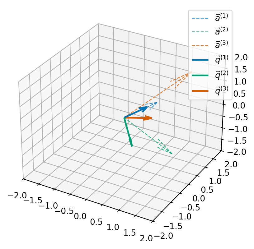
Now we have applied the Gram-Schmidt process to convert from the vectors \(\vec{a}^{(j)}\) to the vectors \(\vec{q}^{(j)}\). We can consider the matrix \(Q\) whose columns are the vectors \(\vec{q}^{(j)}\) and the matrix \(A\) whose columns are the vectors \(\vec{a}^{(j)}\): \[\begin{equation*} Q = \begin{pmatrix} && \\ \vec{q}^{(1)} & \vec{q}^{(2)} & \vec{q}^{(3)} \\ && \end{pmatrix} \quad \text{and} \quad A = \begin{pmatrix} && \\ \vec{a}^{(1)} & \vec{a}^{(2)} & \vec{a}^{(3)} \\ && \end{pmatrix} \end{equation*}\] Then we can compute that \[\begin{align*} (Q^T A)_{ij} = \vec{q}^{(j)} \cdot \vec{a}^{(j)}. \end{align*}\] So \[\begin{align*} (Q^T A) & = \begin{pmatrix} (1, 0, 1)^T \cdot (\tfrac{1}{\sqrt{2}}, 0, \tfrac{1}{\sqrt{2}})^T & (2, -1, 0)^T \cdot (\tfrac{1}{\sqrt{2}}, 0, \tfrac{1}{\sqrt{2}})^T & (1, 2, 1)^T \cdot (\tfrac{1}{\sqrt{2}}, 0, \tfrac{1}{\sqrt{2}})^T \\ (1, 0, 1)^T \cdot (\tfrac{1}{\sqrt{3}}, \tfrac{-1}{\sqrt{3}}, \tfrac{-1}{\sqrt{3}})^T & (2, -1, 0)^T \cdot (\tfrac{1}{\sqrt{3}}, \tfrac{-1}{\sqrt{3}}, \tfrac{-1}{\sqrt{3}})^T & (1, 2, 1)^T \cdot (\tfrac{1}{\sqrt{3}}, \tfrac{-1}{\sqrt{3}}, \tfrac{-1}{\sqrt{3}})^T \\ (1, 0, 1)^T \cdot (\tfrac{1}{\sqrt{6}}, \tfrac{2}{\sqrt{6}}, \tfrac{-1}{\sqrt{6}})^T & (2, -1, 0)^T \cdot (\tfrac{1}{\sqrt{6}}, \tfrac{2}{\sqrt{6}}, \tfrac{-1}{\sqrt{6}})^T & (1, 2, 1)^T \cdot (\tfrac{1}{\sqrt{6}}, \tfrac{2}{\sqrt{6}}, \tfrac{-1}{\sqrt{6}})^T \end{pmatrix} \\ & = \begin{pmatrix} \tfrac{2}{\sqrt{2}} & \tfrac{2}{\sqrt{2}} & \tfrac{2}{\sqrt{2}} \\ 0 & \tfrac{3}{\sqrt{3}} & \tfrac{-2}{\sqrt{3}} \\ 0 & 0 & \tfrac{4}{\sqrt{6}} \end{pmatrix}. \end{align*}\] Hence we have found an upper triangular matrix \(R = Q^T A\). Since \(Q\) is orthogonal, we know \(Q^{-1} = Q^T\) and we have a factorisation: \[\begin{equation*} A = Q R. \end{equation*}\]
Exercise 8.2 Continue the QR-factorisation process by computing \(B = R Q\) and apply the Gram-Schmidt process to the columns of \(B\).
Remark. The Gram-Schmidt algorithm relies on the fact that after each projection there should be something left - i.e. \(\vec{u}^{(j)}\) should be non-zero. If \(\vec{a}^{(j)}\) is in the span of \(\{ \vec{q}^{(1)}, \ldots, \vec{q}^{(j-1)} \}\), then the projection onto \(\vec{u}^{(j)}\) will give \(\vec{0}\). There are a few ways to test this, but the key idea is that if \(A\) is non-singular then we will always have \(\vec{u}^{(j)} \neq \vec{0}\) – at least in exact-precision calculations…
8.1.2 Python QR factorisation using Gram-Schmidt
def gram_schmidt_qr(A):
    """
    Compute the QR factorization of a square matrix using the classical
    Gram-Schmidt process.

    Parameters
    ----------
    A : numpy.ndarray
        A square 2D NumPy array of shape ``(n, n)`` representing the input
        matrix.

    Returns
    -------
    Q : numpy.ndarray
        Orthogonal matrix of shape ``(n, n)`` where the columns form an
        orthonormal basis for the column space of A.
    R : numpy.ndarray
        Upper triangular matrix of shape ``(n, n)``.
    """
    n, m = A.shape
    if n != m:
        raise ValueError(f"the matrix A is not square, {A.shape=}")

    Q = np.empty_like(A)
    R = np.zeros_like(A)

    for j in range(n):
        # Start with the j-th column of A
        u = A[:, j].copy()

        # Orthogonalize against previous q vectors
        for i in range(j):
            R[i, j] = np.dot(Q[:, i], A[:, j])  # projection coefficient
            u -= R[i, j] * Q[:, i]  # subtract the projection

        # Normalize u to get q_j
        R[j, j] = np.linalg.norm(u)
        Q[:, j] = u / R[j, j]

    return Q, R
Let’s test it without our example above:
A = [  1.0,  2.0,  1.0 ]
    [  0.0, -1.0,  2.0 ]
    [  1.0,  0.0,  1.0 ]
QR factorisation:
Q = [  0.70711,  0.57735,  0.40825 ]
    [  0.00000, -0.57735,  0.81650 ]
    [  0.70711, -0.57735, -0.40825 ]
R = [  1.41421,  1.41421,  1.41421 ]
    [  0.00000,  1.73205, -1.15470 ]
    [  0.00000,  0.00000,  1.63299 ]
Have we computed a factorisation? (A == Q @ R?) True
8.2 Finding eigenvalues and eigenvectors
The algorithm given above says that we use the QR factorisation to iteratively find a sequence of matrices \(A^{(j)}\) which should converge to an upper-triangular matrix.
We test this out in code first for the matrix from Example 7.3:
def gram_schmidt_eigen(A, maxiter=100, verbose=False):
    """
    Compute the eigenvalues and eigenvectors of a square matrix using the QR
    algorithm with classical Gram-Schmidt QR factorization.

    This function implements the basic QR algorithm:

    1. Factorize the matrix `A` into `Q` and `R` using Gram-Schmidt QR
       factorization.
    2. Update the matrix as:

       .. math::
           A_{k+1} = R_k Q_k

    3. Accumulate the orthogonal transformations in `V` to compute the
       eigenvectors.
    4. Iterate until `A` becomes approximately upper triangular or until the
       maximum number of iterations is reached.

    Once the iteration converges, the diagonal of `A` contains the eigenvalues,
    and the columns of `V` contain the corresponding eigenvectors.

    Parameters
    ----------
    A : numpy.ndarray
        A square 2D NumPy array of shape ``(n, n)`` representing the input
        matrix. This matrix will be **modified in place** during the
        computation.
    maxiter : int, optional
        Maximum number of QR iterations to perform. Default is 100.
    verbose : bool, optional
        If ``True``, prints intermediate matrices (`A`, `Q`, `R`, and `V`) at
        each iteration. Useful for debugging and understanding convergence.
        Default is ``False``.

    Returns
    -------
    eigenvalues : numpy.ndarray
        A 1D NumPy array of length ``n`` containing the eigenvalues of `A`.
        These are the diagonal elements of the final upper triangular matrix.
    V : numpy.ndarray
        A 2D NumPy array of shape ``(n, n)`` whose columns are the normalized
        eigenvectors corresponding to the eigenvalues.
    it : int
        The number of iterations taken by the algorithm.
    """
    # identity matrix to store eigenvectors
    V = np.eye(A.shape[0])

    if verbose:
        print_array(A)

    it = -1
    for it in range(maxiter):
        if verbose:
            print(f"\n\n{it=}")

        # perform factorisation
        Q, R = gram_schmidt_qr(A)
        if verbose:
            print_array(Q)
            print_array(R)

        # update A and V in place
        A[:] = R @ Q
        V[:] = V @ Q

        if verbose:
            print_array(A)
            print_array(V)

        # test for convergence: is A upper triangular up to tolerance 1.0e-8?
        if np.allclose(A, np.triu(A), atol=1.0e-8):
            break

    eigenvalues = np.diag(A)
    return eigenvalues, V, it
A = np.array([[3.0, 1.0], [1.0, 3.0]])
print_array(A)
eigenvalues, eigenvectors, it = gram_schmidt_eigen(A)
print_array(eigenvalues)
print_array(eigenvectors)
print("iterations required:", it)A = [ 3.0, 1.0 ]
[ 1.0, 3.0 ]
eigenvalues = [ 4.0 ]
[ 2.0 ]
eigenvectors = [ 0.7071, -0.7071 ]
[ 0.7071, 0.7071 ]
iterations required: 27These values agree with those from Example 7.3. Note that this code normalises the eigenvectors to have length one, so we have slightly different values for the eigenvectors but still in the same directions.
8.3 Correctness and convergence
Let’s see what happens when we try this same approach for a bigger symmetric matrix. We write a test that first checks how good the QR factorisation is for the initial matrix \(A\) and then uses our approach to find eigenvalues and eigenvectors and tests how good that approximation is too.
# replicable seed
np.random.seed(42)

for n in [2, 4, 8, 16, 32]:
    print(f"\n\n matrix size {n=}")
    # generate a random matrix
    S = special_ortho_group.rvs(n)
    D = np.diag(np.random.randint(-5, 5, (n,)))
    A = S.T @ D @ S

    Q, R = gram_schmidt_qr(A)

    print(
        "- how accurate is Q R factorisation of A?",
        np.linalg.norm(A - Q @ R),
    )
    print("- is Q orthogonal?", np.linalg.norm(np.eye(n) - Q.T @ Q))

    print("- can we use this approach to find eigenvalues?")
    maxiter = 100_000
    D, V, k = gram_schmidt_eigen(A, maxiter=maxiter)
    if k == maxiter - 1:
        print(" -> too many iterations required")
    else:
        print(
            f" -> are the eigenvalues and eigenvectors accurate? {k=}",
            np.linalg.norm(A @ V - np.diag(D) @ V),
        )
 matrix size n=2
- how accurate is Q R factorisation of A? 1.1102230246251565e-16
- is Q orthogonal? 2.434890684976629e-16
- can we use this approach to find eigenvalues?
 -> are the eigenvalues and eigenvectors accurate? k=26 8.79893075620144e-09


 matrix size n=4
- how accurate is Q R factorisation of A? 4.965068306494546e-16
- is Q orthogonal? 3.316125075834646e-16
- can we use this approach to find eigenvalues?
 -> too many iterations required


 matrix size n=8
- how accurate is Q R factorisation of A? 1.0530671687875234e-15
- is Q orthogonal? 5.922760902330306e-16
- can we use this approach to find eigenvalues?
 -> are the eigenvalues and eigenvectors accurate? k=45 1.498289419704859e-08


 matrix size n=16
- how accurate is Q R factorisation of A? 1.5600199530047478e-15
- is Q orthogonal? 1.2863227488047944
- can we use this approach to find eigenvalues?
 -> too many iterations required


 matrix size n=32
- how accurate is Q R factorisation of A? 3.1345684296560498e-15
- is Q orthogonal? 5.464883404922812
- can we use this approach to find eigenvalues?
 -> too many iterations required
You will see in the lab session ways to improve our basic algorithm that allows faster, more robust convergence.